Difference between revisions of "Signal Processing"
m |
|||
| (18 intermediate revisions by 2 users not shown) | |||
| Line 1: | Line 1: | ||
| − | Signal Processing | + | <!-- CATEGORIES --> |
| − | It is | + | [[Category: Developer's Guide]][[Category:GCube Spatial Data Infrastructure]] |
| + | <!-- CATEGORIES --> | ||
| + | Signal Processing is a set of facilities that aim to analyze signals or measure time-varying or spatially varying physical quantities. It is part of the gCube-system facilities for Data Mining and Processing. It is especially used in order to discover seasonality and periodicity in time series of real valued observations. Such observations can refer, for example, to catch statistics in fisheries, marine species presence occurrence or environmental parameters modulations. The Signal Processing facilities are part of the '''Ecological Engine''' gCube library. This library is responsible for hosting all the basic data processing and mining procedures for biological and environmental datasets. | ||
| + | |||
| + | The Signal Processing facilities especially aim at facing the following issues: | ||
| + | * Reconstruct a uniformly sampled time series from a non-uniform time series | ||
| + | * Perform Short-Time Standard Fourier Analysis | ||
| + | * Trace the Spectrogram of a Time Series | ||
| + | * Highlight periodicity in a Time Series | ||
== Overview == | == Overview == | ||
| + | Signal Processing is used in many ways by the gCube based e-Infrastructures. GIS layers, containing geographical information, can report the variations of some environmental parameters in time. Information can be stored in NetCDF files as well as on remote GeoServers. Geographical maps can contain information about environmental parameters distributions or species distributions, but these are usually not uniformly defined. At some point, in time and space, values can be missing. For such reasons, the '''Ecological Engine''' library puts together data mining techniques and Signal Processing facilities in order to fill the gaps, reconstruct signals and produce time-frequency analysis. | ||
== Features == | == Features == | ||
| − | + | The features currently supported by the Signal Processing facilities include: | |
| − | + | ||
| + | * signal reconstruction: rebuilds a time series which is not uniformly sampled in time; | ||
| + | * spectrogram calculation and display: produces the spectrogram of a signal with the Short-Time Fourier Transform (STFT) technique, according to a certain sampling frequency and time-window shift; | ||
| + | * multi-signal analysis by means of summed spectrogram: analyzes several synchronized signals and produces a spectrogram which is the sum of the single spectrograms; | ||
| + | * delta + double delta features: produces the delta and double delta features, related to the first and second derivative of the signal; | ||
| + | * center frequency calculation: calculates the central frequency in a filterbank; | ||
| + | * cepstral coefficients calculation: calculates the cepstral coefficients of a signal, which store much of the information contained in the signal; | ||
| + | * spectrum frequency band cut: cuts the signal spectrum according to a certain frequency band; | ||
| + | * filterbanks: produces a filterbank for filtering the signal in complex way; | ||
| + | * mel filterbanks: builds a perceptually inspired filterbank based on the mel frequencies distribution. | ||
| + | |||
| + | A set of utilities are included in the '''Ecological Engine''' library in order to perform the above operations: | ||
| + | * linear frequency to mel frequency tranformation | ||
| + | * frequency to index in Short-Time Fourier Transform | ||
| + | * transformation to and from Rapid Miner Example Set | ||
| + | * sinusoid signal generation | ||
| + | * inverse mel calculation | ||
| + | * sample to time and time to sample conversions | ||
| + | * signal timeline generation | ||
| + | * index to time conversion for spectrograms | ||
| + | * time to index conversion for spectrograms | ||
| + | |||
| + | == Software == | ||
| + | The software is available on the gCube maven repository by including the following component in the pom.xml file: | ||
| + | |||
| + | <source lang="java"> | ||
| + | <dependency> | ||
| + | <groupId>org.gcube.dataanalysis</groupId> | ||
| + | <artifactId>ecological-engine</artifactId> | ||
| + | <version>1.6.1-SNAPSHOT</version> | ||
| + | </dependency> | ||
| + | </source> | ||
| + | |||
| + | An example to call the spectrogram analysis with STFT and produce the chart is: | ||
| + | |||
| + | <source lang="java"> | ||
| + | SignalConversions.spectrogram(name, signal, samplingRate, windowshift, frameslength, display) | ||
| + | </source> | ||
| + | |||
| + | Where the input variables are: | ||
| + | <source lang="java"> | ||
| + | String name: the title of the chart | ||
| + | double[] signal: the sequence of values representing the trend | ||
| + | int samplingRate: the sampling frequency in integer value and multiple of 2 | ||
| + | int windowshift: the window shift of the STFT in samples | ||
| + | int frameslength: the length of each window in samples | ||
| + | boolean display: a flag to ask the procedure to run an applet which displays the spectrogram | ||
| + | </source> | ||
| + | |||
| + | An example which performs a signal reconstruction is: | ||
| + | |||
| + | <source lang="java"> | ||
| + | AlgorithmConfiguration config = new AlgorithmConfiguration(); | ||
| + | config.setConfigPath(configDir); | ||
| + | config.initRapidMiner(); | ||
| + | SignalProcessing.fillSignal(signal) | ||
| + | </source> | ||
| + | |||
| + | where the input parameters are defined as follows: | ||
| + | |||
| + | <source lang="java"> | ||
| + | double[] signal: the sequence of values representing the trend | ||
| + | String configDir: a configuration folder containing the configuration files required by the Ecological Engine library | ||
| + | </source> | ||
| + | |||
| + | The cfg directory and the Ecological Engine library are accessible at this svn link: http://svn.research-infrastructures.eu/d4science/gcube/trunk/data-analysis/EcologicalEngine | ||
| + | |||
| + | == Experiments == | ||
| + | In the following experiments we give the idea of the transformations and processing that can be applied to signals by means of the Signal Processing (SP) facilities included in the '''Ecological Engine'' library. | ||
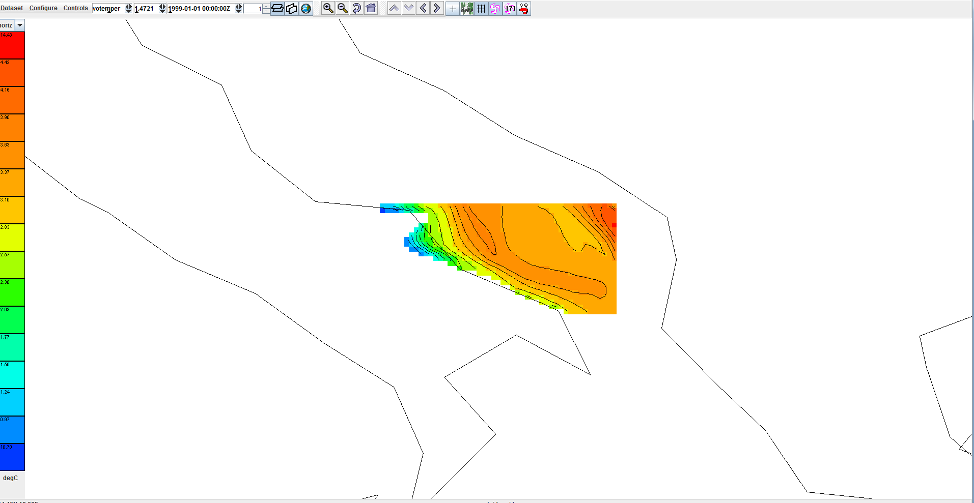
| + | We selected a study area around Bari, Italy (ref. Fig. 1). | ||
| + | [[File:Bari.png|700px|thumb|center|Figure 1. A study area around Bari, Italy.]] | ||
| + | |||
| + | We then extracted the temperature time series from a point in that area with coordinates (17.59;41.37). We downloaded a NetCDF file from the MyOceans repository, which contained mean monthly variations for the sea surface temperature between the years 2000 and 2010. By using the geographical extraction facilities of gCube for the NetCDF files, we extracted the time trend of the temperature. By using the Signal Processing facilities we produced the chart in Fig. 2. | ||
| + | |||
| + | [[Image:Temperature.png|700px|thumb|center|Figure 2. Variation of sea surface temperature between the years 2000 and 2010 in the point (17.59;41.37).]] | ||
| − | + | We used the spectrogram generation facility to produce the spectrogram plot of the signal (ref. Fig. 3). A continuous line is evident around 2.5E-8 Hz, which corresponds approximately to 12.2 months. | |
| + | [[File:TemperatureSpectrogram.png|700px|thumb|center|Figure 3. Spectrogram of the monthly temperature trend between the years 2000 and 2010 in the point (17.59;41.37).]] | ||
| − | + | The simple spectrogram produced by the STFT was then able to underline a hidden periodicity in the trend. | |
| − | + | ||
| − | + | ||
| − | + | ||
| − | + | ||
| − | + | ||
| − | + | ||
| − | + | ||
| − | + | ||
| − | + | As further example, we report the usage of the gCube SP facilities on a signal that is not uniformly sampled in time. We took the trend of some earthquakes report for the region of Garfagnana (Tuscany, Italy) by the INGV institute (www.ingv.it). The points are not equally spaced in time, which means that the trend is not uniformly sampled. | |
| − | + | ||
| − | + | ||
| − | + | ||
| − | + | ||
| − | + | ||
| − | + | ||
| − | + | ||
| − | + | ||
| − | time | + | |
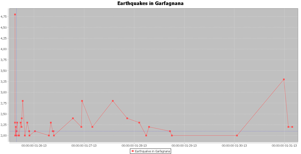
| + | [[File:Earthquakes.png|700px|thumb|center|Figure 4. Trend of the earthquakes in Garfagnana at the beginning of 2013. The trend is not uniformly sampled.]] | ||
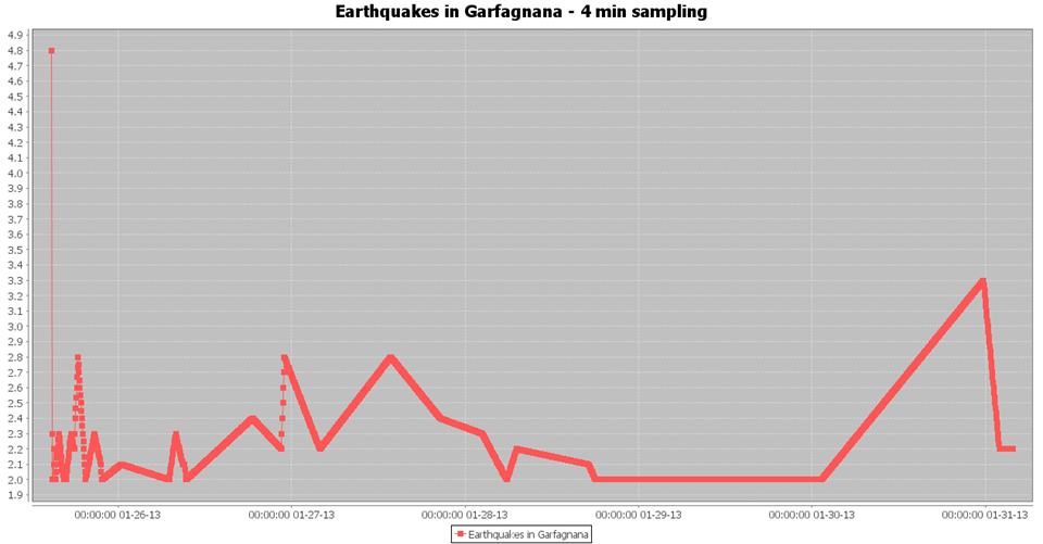
| − | [[ | + | By applying a K-Nearest Neighbor data mining process, we were able to reconstruct the signal at the missing points. We simulated a sampling of 4 minutes and eventually obtained the trend in Fig. 5. |
| + | [[File:EarthquakesReconstructed.png|700px|thumb|center|Figure 5. Reconstructed trend of the earthquakes with 4 minutes of time sampling.]] | ||
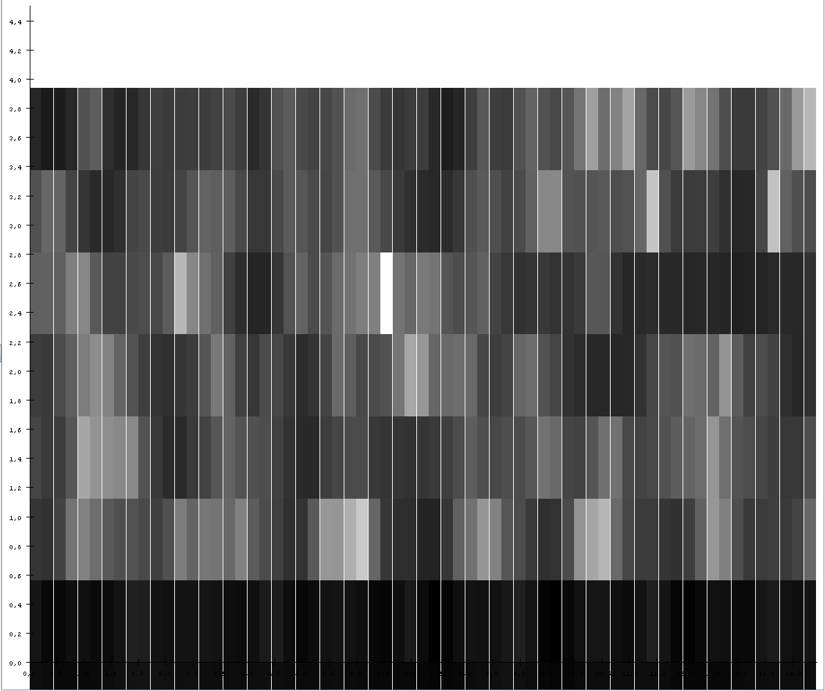
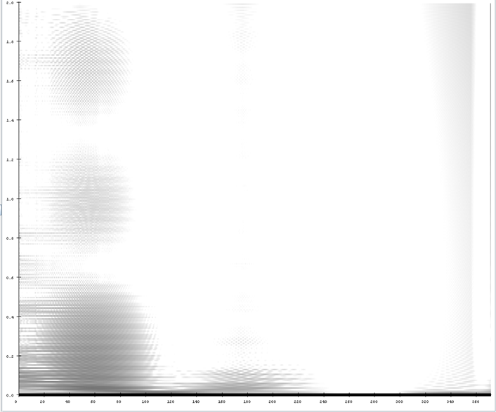
| − | [[ | + | At such point we could produce the spectrogram of the reconstructed signal. The surprising fact is that it highlights three well defined periods hidden in the first part of the signal. The correspondent frequencies are superposed in the same time period (ref. Fig. 4). |
| + | [[File:EarthquakesSpectrogram.png|700px|thumb|center|Figure 6. Spectrogram of the earthquakes trend. Three hidden periods are detected by the STFT.]] | ||
Latest revision as of 14:52, 6 July 2016
Signal Processing is a set of facilities that aim to analyze signals or measure time-varying or spatially varying physical quantities. It is part of the gCube-system facilities for Data Mining and Processing. It is especially used in order to discover seasonality and periodicity in time series of real valued observations. Such observations can refer, for example, to catch statistics in fisheries, marine species presence occurrence or environmental parameters modulations. The Signal Processing facilities are part of the Ecological Engine gCube library. This library is responsible for hosting all the basic data processing and mining procedures for biological and environmental datasets.
The Signal Processing facilities especially aim at facing the following issues:
- Reconstruct a uniformly sampled time series from a non-uniform time series
- Perform Short-Time Standard Fourier Analysis
- Trace the Spectrogram of a Time Series
- Highlight periodicity in a Time Series
Contents
Overview
Signal Processing is used in many ways by the gCube based e-Infrastructures. GIS layers, containing geographical information, can report the variations of some environmental parameters in time. Information can be stored in NetCDF files as well as on remote GeoServers. Geographical maps can contain information about environmental parameters distributions or species distributions, but these are usually not uniformly defined. At some point, in time and space, values can be missing. For such reasons, the Ecological Engine library puts together data mining techniques and Signal Processing facilities in order to fill the gaps, reconstruct signals and produce time-frequency analysis.
Features
The features currently supported by the Signal Processing facilities include:
- signal reconstruction: rebuilds a time series which is not uniformly sampled in time;
- spectrogram calculation and display: produces the spectrogram of a signal with the Short-Time Fourier Transform (STFT) technique, according to a certain sampling frequency and time-window shift;
- multi-signal analysis by means of summed spectrogram: analyzes several synchronized signals and produces a spectrogram which is the sum of the single spectrograms;
- delta + double delta features: produces the delta and double delta features, related to the first and second derivative of the signal;
- center frequency calculation: calculates the central frequency in a filterbank;
- cepstral coefficients calculation: calculates the cepstral coefficients of a signal, which store much of the information contained in the signal;
- spectrum frequency band cut: cuts the signal spectrum according to a certain frequency band;
- filterbanks: produces a filterbank for filtering the signal in complex way;
- mel filterbanks: builds a perceptually inspired filterbank based on the mel frequencies distribution.
A set of utilities are included in the Ecological Engine library in order to perform the above operations:
- linear frequency to mel frequency tranformation
- frequency to index in Short-Time Fourier Transform
- transformation to and from Rapid Miner Example Set
- sinusoid signal generation
- inverse mel calculation
- sample to time and time to sample conversions
- signal timeline generation
- index to time conversion for spectrograms
- time to index conversion for spectrograms
Software
The software is available on the gCube maven repository by including the following component in the pom.xml file:
<dependency>
  <groupId>org.gcube.dataanalysis</groupId>
  <artifactId>ecological-engine</artifactId>
  <version>1.6.1-SNAPSHOT</version>
</dependency>
An example to call the spectrogram analysis with STFT and produce the chart is:
SignalConversions.spectrogram(name, signal, samplingRate, windowshift, frameslength, display)
Where the input variables are:
String name: the title of the chart
double[] signal: the sequence of values representing the trend
int samplingRate: the sampling frequency in integer value and multiple of 2
int windowshift: the window shift of the STFT in samples
int frameslength: the length of each window in samples
boolean display: a flag to ask the procedure to run an applet which displays the spectrogram
An example which performs a signal reconstruction is:
AlgorithmConfiguration config = new AlgorithmConfiguration();
config.setConfigPath(configDir);
config.initRapidMiner();
SignalProcessing.fillSignal(signal)
where the input parameters are defined as follows:
double[] signal: the sequence of values representing the trend
String configDir: a configuration folder containing the configuration files required by the Ecological Engine library
The cfg directory and the Ecological Engine library are accessible at this svn link: http://svn.research-infrastructures.eu/d4science/gcube/trunk/data-analysis/EcologicalEngine
Experiments
In the following experiments we give the idea of the transformations and processing that can be applied to signals by means of the Signal Processing (SP) facilities included in the 'Ecological Engine library. We selected a study area around Bari, Italy (ref. Fig. 1).
We then extracted the temperature time series from a point in that area with coordinates (17.59;41.37). We downloaded a NetCDF file from the MyOceans repository, which contained mean monthly variations for the sea surface temperature between the years 2000 and 2010. By using the geographical extraction facilities of gCube for the NetCDF files, we extracted the time trend of the temperature. By using the Signal Processing facilities we produced the chart in Fig. 2.
We used the spectrogram generation facility to produce the spectrogram plot of the signal (ref. Fig. 3). A continuous line is evident around 2.5E-8 Hz, which corresponds approximately to 12.2 months.
The simple spectrogram produced by the STFT was then able to underline a hidden periodicity in the trend.
As further example, we report the usage of the gCube SP facilities on a signal that is not uniformly sampled in time. We took the trend of some earthquakes report for the region of Garfagnana (Tuscany, Italy) by the INGV institute (www.ingv.it). The points are not equally spaced in time, which means that the trend is not uniformly sampled.
By applying a K-Nearest Neighbor data mining process, we were able to reconstruct the signal at the missing points. We simulated a sampling of 4 minutes and eventually obtained the trend in Fig. 5.
At such point we could produce the spectrogram of the reconstructed signal. The surprising fact is that it highlights three well defined periods hidden in the first part of the signal. The correspondent frequencies are superposed in the same time period (ref. Fig. 4).
